Graph the Set of Data Draw a Trend Line

PYTHON

Level Up Your Data Visualizations with Trend Lines in Python

Using the Plotly library to easily visualize trends in your data

Artwork by my talented sister

Data visualization is a key part of data analysis. Visualizing data makes it easier for people to understand the trends in a dataset compared to just looking at numbers on a table. Part of this includes picking the right chart types to go with the right type of data you are trying to showcase, like using a line chart for time-series data.

You can go further than this by adding some cosmetic changes like color and font to make important data points pop. In addition, trend lines are helpful to clearly outline the general direction of a dataset over all its data points. You could also implement static trend lines to have a value you choose to be a horizontal or vertical line on the graph that you use to easily see if the values in your dataset are higher or lower than the static line.

In this piece, we will take a look at implementing both forms of trend lines using the Plotly library in Python for the data visualization. We'll also use Pandas for some initial data pre-processing, so make sure you have these two packages installed already. Then, import the following and get ready to follow along!

            import pandas as pd
import plotly.express as px
import random          

Let's get to it!

Creating a line chart with an average trend line with Plotly

Let's first generate some sample data. To do so, run the following code.

            expense_data = {
              "Person": random.choices(["A", "B"], k=20),
              "Amount": random.sample(range(100, 200), 10) + random.sample(range(0, 99), 10),
              "Category": ["Groceries"] * 10 + ["Restaurant"] * 10,
              "Date": pd.to_datetime(pd.date_range('2020-01-01','2020-10-01', freq='MS').tolist() * 2)
}
df = pd.DataFrame(data=expense_data)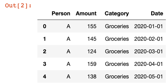          

The data we're going to visualize will be based on some randomly generated personal expense data. Above you can see we're just randomly creating expense data for 10 months and loading it into a Pandas DataFrame. The above code should output 20 lines worth of data.

In this piece, the first goal of our data analysis is to compare the average monthly spending per category to each month's spending in that category.

As such, let's use some Pandas to group the total spending per month together per category.

            df_grouped = df.groupby(by=[pd.Grouper(key="Date", freq="1M"), "Category"])["Amount"]
df_grouped = df_grouped.sum().reset_index()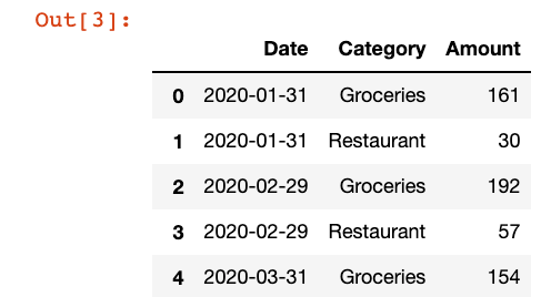          

Now, we can get to creating charts.

Since we want to create a chart for each category of spending with each of its monthly data points and a static average trend line, we can start by creating a list of the categories in our DataFrame.

            categories = df["Category"].unique().tolist()          

Then, we'll loop through all the categories and create a graph for each using the following code.

            for category in categories:
              df_category = df_grouped.loc[df_grouped["Category"] == category].copy()
              df_category["Average Spending"] = round(df_category["Amount"].mean(), 2)
              category_graph = px.line(
              df_category,              
              x="Date",              
              y=["Amount", "Average Spending"],              
              title=f"{category} Spending with Average Trend Line"
              )
              category_graph.show()          

This code first creates a new DataFrame with only the rows that have the desired category in each loop. Then, we create a new column "Average Spending" which simply uses the mean method on the "Amount" column in the DataFrame to return a column with only the average spending values.

Finally, we use the Plotly Express library to create a line chart with the new DataFrame. You'll notice that we passed a list into the y parameter, which will give us two lines in the line chart. The result of this code is the following graphs.

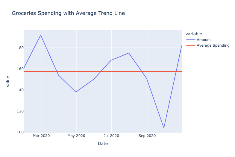
Using these graphs, you can easily see which months fall over the average spending for the category and which are under. This would be helpful for someone looking to manage their finances over time so that they could budget each month accordingly and check to see if they're meeting their plans every month.

Implementing linear and non-linear trend lines on graphs with Plotly

Next, let's take a look at using Plotly to create trend lines for the total monthly spending in the dataset. To do so, we'll create a new grouped DataFrame, only this time we only need to group it by the month.

            df_sum = df.groupby(by=[pd.Grouper(key="Date", freq="1M")])["Amount"]
df_sum = df_sum.sum().reset_index()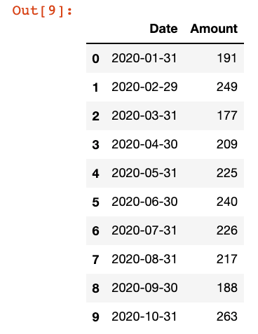          

Plotly allows you to create both linear or non-linear trend lines. You can use ordinary least squares (OLS) linear regression or locally weighted scatterplot smoothing (non-linear) trend lines.

Similar to how we created the graphs for the previous sections, we'll now create a list of the possible trend lines and create scatter plots with Plotly using another for loop.

            trend_lines = ["ols", "lowess"]            for trend_line in trend_lines:
              fig = px.scatter(
              df_sum,              
              x="Date",
              y="Amount",
              trendline=trend_line,
              title=f"{trend_line} Trend Line"
              )
              fig.show()          

The code is more or less the same as before, where we pass in the DataFrame and the appropriate columns to the Plotly Express scatterplot. To add the trend lines, we pass in each trend line value from the list we defined into the trendline argument. Running the above code will give you the following graphs.

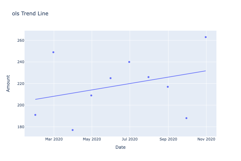
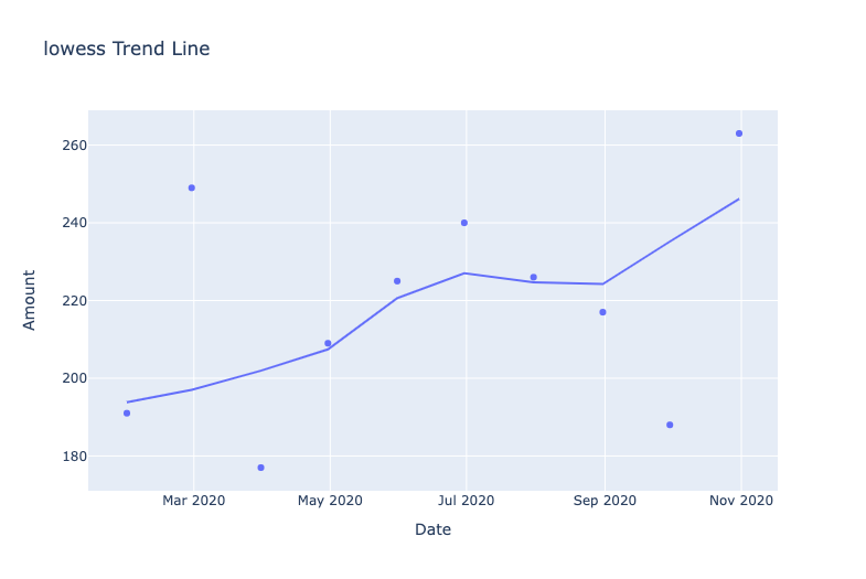
Depending on your dataset, a linear or non-linear trend line can better fit the data points. That's why it's useful to try different trendlines to see which one fits the data better. Also, just because there is a trend line does not necessarily mean that a trend is really there (in the same way that correlation does not equal causation). You can also access the model parameters (for charts with an OLS trend line) using the following code.

            results = px.get_trendline_results(fig)
results.px_fit_results.iloc[0].summary()          

Note that the fig object above is specifically the figure created where the trendline argument in the Plotly Express scatter is set to "ols". The result of the summary can provide you with an explanation of the parameters used to create the trend line you see in the chart, which can help you understand the significance of the trend line.

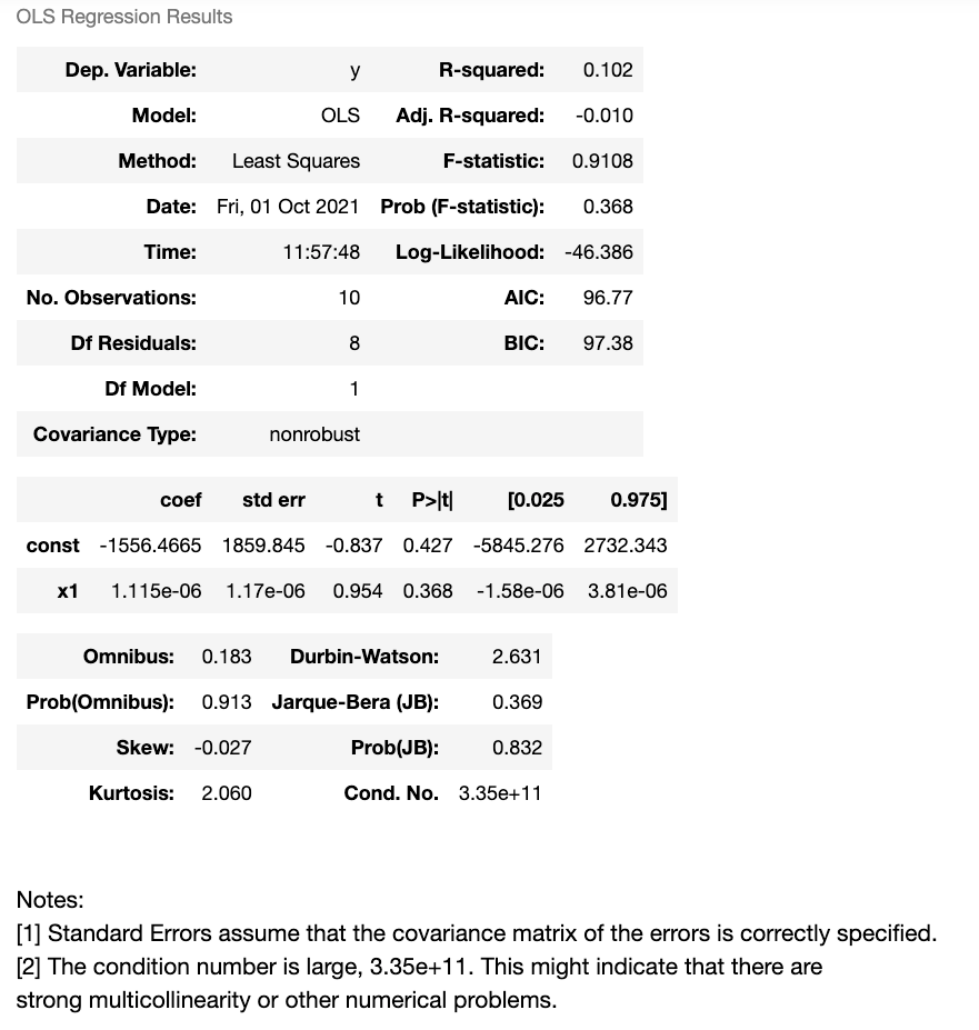
In our case with randomly generated data, it's a bit difficult to really see a significant trend. You'll see the very low R-squared value and a sample size of less than 20 imputes a low correlation (if any at all).

However, for a regular person's expense data, it would be great to see a trend line that's mostly flat when you look at the spending per month. If you notice a highly sloped positive trend line with a higher R-squared value in your monthly expenses, you would know that you may have increased your spending over time and therefore are spending more than your monthly budget allocation (unless maybe you got a raise and decided to splurge on purpose).

Graph the Set of Data Draw a Trend Line

Source: https://towardsdatascience.com/level-up-your-data-visualizations-with-trend-lines-in-python-6ad4a8253d6

Share this post